Chem1 General Chemistry Virtual Textbook → acid-base equilibria → Buffers
Mixtures of conjugate acids and bases
How the pH controls composition; buffers
On this page:
- 1 pH as a controlling variable
- 2 Buffer solutions
- The Henderson-Hasselbalch eqn.
- Practical buffer calculations
- Pitfalls of the H-H equation
- Effectiveness of buffers; buffer index, buffer capacity
- 3 log-C (Sillén) plots
- Simple example: the acetate system
- Ammonia - a weak base
- Understanding the plots: the proton condition
- Ammonium acetate - a salt
- Polyprotic systems
- 4 How to draw Sillén diagrams
- What you should be able to do
- Some useful references
- Some worthwhile videos
We often tend to regard the pH as a quantity that is dependent on other variables such as the concentration and strength of an acid, base or salt. But in much of chemistry (and especially in biochemistry), we find it more useful to treat pH as the "master" variable that controls the relative concentrations of the acid- and base-forms of one or more sets of conjugate acid-base systems.
In this lesson, we will explore this approach in some detail, showing its application to the very practical topics of buffer solutions, as well as the use of a simple graphical approach that will enable you to estimate the pH of a weak monoprotic or polyprotic acid or base without doing any arithmetic at all!
Some ![]() videos are can be found near the bottom of this page.
videos are can be found near the bottom of this page.
Note that because we are discussing stoichiometry here, we are interested in quantities (moles) of reactants, not concentrations of reactants.
If we add 0.2 mol of sodium hydroxide to a solution containing 1.0 mol of a weak acid HA, then an equivalent number of moles of that acid will be converted into its base form A–. The resulting solution will contain 0.2 mol of A– and 0.8 mol of HA.
The important point to understand here is that we will end up with a “partly neutralized” solution in which both the acid and its conjugate base are present in significant amounts. Solutions of this kind are far more common than those of a pure acid or a pure base, and it is very important that you have a thorough understanding of them.
To a solution containing 0.010 mole of acetic acid (HAc), we add 0.002 mole of sodium hydroxide. If the volume of the final solution is 100 ml, find the values of Ca, Cb, and the total system concentration Ct.
Solution: The added hydroxide ion, being a strong base, reacts completely with the acetic acid, leaving .010 – .002 = .008 mole of HAc and .002 mole of acetate ion Ac–. The final concentrations are Ca = .008 mol / 0.10 L = .08 M,
Cb = .002 mol / 0.10 L = .02 M, Ct = .010 mol / 0.10 L = 0.10 M.
Note that this solution would be indistinguishable from one prepared by combining Ca = .080 mole of acetic acid with Cb = 0.020 mole of sodium acetate and adjusting the volume to 100 ml.
Thus starting with a solution of a pure weak acid or weak base in water, we can add sufficient strong base or strong acid, respectively, to adjust the ratio of the conjugate species — that is, the ratios [HA]/[A–] in the case of an acid, or [B]/[BH+] for a base, to any value we want.
Ionization fractions
In order to express the relative concentrations of the protonated and deprotonated forms of an acid-base system present in a solution, we could use the simple ratio [HA]/[A] (or its inverse), but this suffers from the drawback of yielding an indeterminate result when the concentration in the denominator is zero. For many purposes it is more convenient to use the ionization fractions

(1-7)
The fraction![]() 1 is also known as the degree of dissociation of the acid. By making appropriate substitutions using the relation
1 is also known as the degree of dissociation of the acid. By making appropriate substitutions using the relation
 (1-8)
(1-8)
we can express the ionization fractions as functions of the pH:
 (1-9)
(1-9)
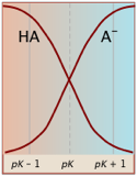
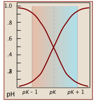
Notice (left) that the the values for both of these functions are close to zero or unity except within the pH range pKa ± 1.
Gallery of ionization fraction plots
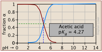
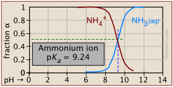
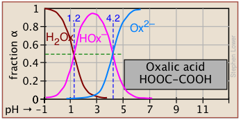
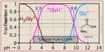
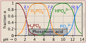
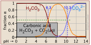
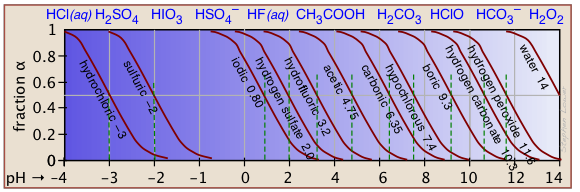
Plots of the![]() functions vs pH for several systems are shown below. Notice the crossing points where [HA] = [A] when [H+] = Ka. This corresponds to unit value of the quotient in the Henderson-Hasselbalch equation.
functions vs pH for several systems are shown below. Notice the crossing points where [HA] = [A] when [H+] = Ka. This corresponds to unit value of the quotient in the Henderson-Hasselbalch equation.
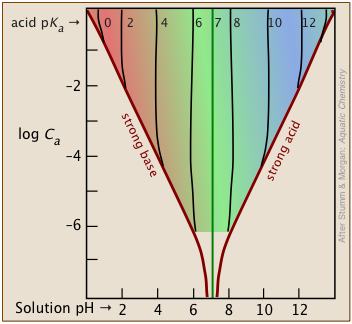
Bird's-eye view
The ionization fractions of a series of acids (but not their ampholytes) over a wide pH range can conveniently be summarized as shown below.
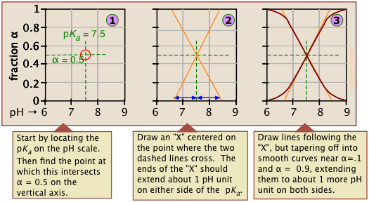
Make your own ionization fraction plots
If you know the pKa of an acid, you can easily sketch out its ionization fraction plot. The extreme tops and bottoms can only be estimated, but the rest of the plots are essentially straight lines.
Limitations of ionization plots
As valuable as these plots are for showing how the distribution of conjugate species varies with the pH, they suffer from two drawbacks:
- Plots of
 cover only a single order of magnitude, but the actual concentrations, which we are often more interested in, vary over a far greater range from pH 0 to 14.
 - They are of little help if one wishes to estimate the pH of a solution of the acid or base, or of one of its salts.
Both of these limitations are readily overcome by the use of easily-constructed logarithmic plots which we describe in the following section.
What is a buffer?
The word buffer has several meanings in English, most of them referring (in its verb form) to cushion, shield, protect, or counteract an adverse effect. In chemistry, it refers specifically to a solution that resists a change in pH when acid or base is added.
A buffer (or buffered) solution is one that resists a change in its pH when H+ or OH– ions are added or removed owing to some other reaction taking place in the same solution. Buffer solutions are essential components of all living organisms.
- Our blood is buffered to maintain a pH of 7.4 that must remain unchanged as metabolically-generated CO2 (carbonic acid) is added and then removed by our lungs.
- Buffers in the oceans, in natural waters such as lakes and streams, and within soils help maintain their environmental stability against acid rain and increases in atmospheric CO2.
- Many industrial processes, such as brewing, require buffer control, as do research studies in biochemistry and physiology that involve enzymes, are active only within certain pH ranges.
How buffers work
The essential component of a buffer system is a conjugate acid-base pair whose concentration is fairly high in relation to the concentrations of added H+ or OH– it is expected to buffer against. A simple buffer system might be a 0.2 M solution of sodium acetate; the conjugate pair here is acetic acid HAc and its conjugate base, the acetate ion Ac–.
The idea is that this conjugate pair "pool" will be available to gobble up any small (≤ 10–3 M) addition of H+ or OH– that may result from other processes going on in the solution.
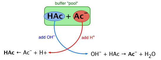
Exercise: sketch out a similar diagram showing what happens when you remove H+ or OH–.
When this happens, the ratio [HAc]/[Ac–],
will remain substantially unchanged, as will the pH, as you will see below.
You can also think of the process depicted above in terms of the LeChâtelier principle: addition of H+ to the solution suppresses the dissociation of HAc, partially counteracting the effect of the added acid, as illustrated by the equation at the bottom left of the above diagram.
The Henderson-Hasselbalch equation
The development given here was also briefly shown in an earlier lesson.
In order to develop this more quantitatively, we will consider the general case of a weak acid HA to which a quantity Cb of strong base has been added; think, for example, of acetic acid which has been partially neutralized by sodium hydroxide, yielding the same conjugate pair described above, although not necessarily identical concentrations.
The mass balance for such a system would be
[HA] + [A–] = Ca + Cb = CT(2-1)
in which Ct denotes the total concentration of all species in the solution. Because we added a strong (completely dissociated) base NaOH to the acid, we also note that
Cb = [Na+] (2-2)
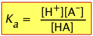
Recalling the equilibrium expression for a weak acid
It is interesting to note that the H-H equation was not developed by chemists!
Lawrence Henderson (1878-1942) was an American medical doctor who taught at Harvard and who studied the acidity of blood and its relation to respiration. In 1908 he worked out the relation shown in Eq. 2-3.
In 1916, K. Hasselbalch, a physiologist at U. of Copenhagen, derived the logarithmic form
(2-6).
You may wonder why these two equations, whose derivation we now consider almost trivial, should have immortalized the names of these two scientists.
The answer is that the theory of chemical equilibrium was still developing in the early 1900's, and had not yet made its way into chemistry textbooks. Even the concept of pH was unknown until Sørenson's work appeared in 1909.
It was the mystery (and medical necessity) of understanding why shortness of breath made the blood more alkaline, and too-rapid breathing made it more acidic, that forced the work of H&H into modern Chemistry.
There is a brief overview of acid-base physiology in lesson 6 of this series.
 (2-3)
(2-3)
We can solve this for [H+]:
![]() (2-4)
(2-4)
Re-writing this in terms of negative logarithms, this becomes
![]() (2-5)
(2-5)
or, since pKa = – log Ka, we invert the ratio to preserve the positive sign:
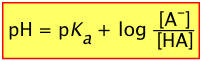 (2-6)
(2-6)
This extremely important relation is known as the Henderson-Hasselbalch equation. It tells us that the pH of a solution containing a weak acid-base system controls the relative concentrations of the acid and base forms of that system.
Of special interest is the case in which the pH of a solution of an acid-base system is set to the value of its pKa. According to the above equation, when pH = pKa, the log term becomes zero, so that the ratio
[AB–] / [HA] = 100 = 1, meaning that [HA] = [AB–]. In other words,
When the pH of a solution is set to the value of the pKa of an acid-base pair, the concentrations of the acid- and base forms will be identical.
This condition can be represented schematically on a proton-free energy diagram:
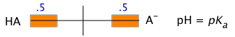
This says, in effect, that at when the pH of a solution containing both the acid and it conjugate baseis made identical to the acid pKa, the forms HA and A– possess identical free energies, and will therefore be present in equal concentrations.
Making and using buffer solutions
Selecting the buffer system
Buffers are generally most effective when the buffer system pKa is not too far from the target pH. Under these conditions, both [HA] and [A–] are large enough to compensate for the withdrawal or addition, respectively, of hydrogen ions.
| acid | formulas | pKa | pH range |
|---|---|---|---|
| phosphoric | H2PO4 / HPO4– | 2.16 | 1-3 |
| carbonic | H2CO3* / HCO3– | 3.75 | 3-5 |
| acetic | HCOOH / HCOO– | 4.75 | 4-6 |
| dihydrogen phosphate | H2PO4– / HPO42– | 7.21 | 6-8 |
| boric | H3BO3 / H2BO3– | 9.24 | 8-10 |
| ammonium | NH4+ / NH3 | 9.25 | 8-10 |
| bicarbonate | HCO3– / CO32– | 10.3 | 9-11 |
| monohydrogen phosphate | HPO42– / PO43– | 12.3 | 11-13 |
Practical buffer calculations
Eq (2-4) above and its logarithmic equivalent (2-6) are of limited use in calculations because the exact values [A–] and [HA] are known only for the special case when the pH of the solution is identical to the pKa. Most buffer solutions will be adjusted to other pH's, and of course, once the buffered solution begins doing it work by counteracting the effect of additions of H+ or OH–, both [A–] and [HA] will have changed.
These two equations are so widely used in practical chemistry (and especially in biochemistry) that they are worth committing to memory.
If you find it difficult to remember which of Ca and Cb go in the top or bottom part of the fraction, or whether the sign in the log form is + or –, you only need to recall that addition of an acid to a buffered solution increases [H+] and decreases the pH. So you can always arrange the equation to make it come out right.
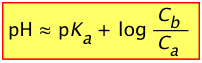
For these reasons, it is useful to rewrite the above two equations by replacing the equilibrium concentrations [A–] and [HA] with the known initial values Ca and Cb:
 (2-7)
(2-7)
 (2-8)
(2-8)
Although these are approximations, they are usually justified because useful buffer systems are always significantly more concentrated than those responsible for adding or removing hydrogen ions. Also, at these higher ionic concentrations, the Ka of the buffer system will seldom be precisely known anyway. Don't expect actual buffer pH's to match calculations to better than 5%.
Compare the effects of adding 1.0 mL of 2.5 M HCl to
a) 100 mL of pure water
b) 100 mL of 0.20 M sodium dihydrogen phosphate solution.
Solution:
a)
- quantity of HCl added: (1.0 mL) × (2.5\ mM/mL) = 2.5 mMol = 0.0025 mol
- concentration of H+ in solution: (.0025 mol) ÷ (.101 L) = .025 M
- pH = – log (.025) = 1.60, change in pH = 1.60 – 7.00 = –5.4
b) (From table immediately above, pKa of H2PO4– is 7.21)
- Initial Ca (H2PO4–) = Cb (HPO42–) = 0.20 M
- Initial pH of buffer solution: pH = pKa + log (Cb/Ca) = 7.21 + 0 = 7.21
- Added HCl will convert .0025 mol of HPO42– to H2PO4–,
changing Ca to (.20 + .0025) mol ÷ (.101 L) = 2.00 M, and
reducing Cb to (.20 – .0025) mol ÷ (.101 L) = 1.95 M - Resulting pH = 7.21 + log (1.95 / 2.00) = 7.21 –.011 = 7.00
- Change in pH = 7.00 – 7.21 = –.21
Note that in both cases the pH is reduced (as it must be if we are adding acid!), but the change is far less in the buffered solution.
How would you prepare 200 mL of a buffer solution whose pH is 9.0?
Solution: The first step would be to select a conjugate acid-base pair whose pKa is close to the desired pH. Looking at the above table of pKa values, either boric acid or ammonium ion would be suitable. For this example, we will select the NH4+/NH3 system, Ka = 5.5E–10, pKa = 9.25.
2) We will use Eq 2-7 (above) to determine the ratio Ca/Cb required to set [H+] to the desired value of 1.00 × 10⁻⁹. To do this, write out the complete equilibrium constant expression for the acid NH4+: NH4+ → NH3 + H+,
and then solve it to find the required concentration ratio:

![]()
3) The easiest (if not particularly elegant) way to work this out is to initially assume that we will dissolve 1.00 mole of solid NH4Cl in water, add sufficient OH– to partially neutralize some of this acid according to the reaction equation
NH4+ + OH– → NH3 + H2O, and then add sufficient water to make the volume
1.00 L.
mass of ammonium chloride: (1 mol) \× (53.5 g Mol) = 53.8 g
let x = moles of NH4+ that must be converted to NH3.
Then Ca/Cb = (1-x)/x = .55; solving this gives x = .64, 1–x = .36.
4) So to make 1 L of the buffer, dissolve .36 × 53.8 g = 19.3 g of solid NH4Cl in a small quantity of water. Add .64 mole of NaOH (most easily done from a stock solution), and then sufficient water to make 1.00 L.
5) To make 200 mL of the buffer, just multiply each of the above figures by 0.200.
Pitfalls of the Henderson-Hasselbalch equation
The H-H equation will be found in virtually all chemistry and biochemistry textbooks and is widely used in practical calculations. What most books do not tell you is that Eq 2-4 is no more than an “approximation of an approximation” which can give incorrect and misleading results when applied to situations in which the simplifying assumptions are not valid.
An exact treatment of conjugate acid-base pairs, including a correct derivation of the Henderson-Hasselbalch equation, is given in the chapter on Exact Calculations.
The H-H equation is only valid for fairly high concentrations
The approximations that lead to the H-H equation limit its reliable use to values of Ca and Cb that are within an order of magnitude of each other, and are fairly high. Also, the pKa of the acid should be moderate.
The shaded portion of this set of plots indicates the values of Ca and Ka that yield useful results. Clearly, the smaller the buffer concentration, the narrower the range of useable acid pKas.
Most buffer solutions tend to be fairly concentrated, with Ca and Cb typically around .01 - 0.1 M.
Thus a buffer based on a .01 M solution of an acid such as chloric (HClO3) with pKa of 1.9 will fall just outside the "safe" boundary near the upper left part of the diagram.
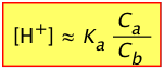
Be careful about confusing the two relations
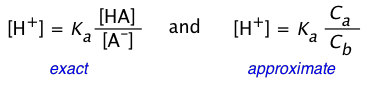 (2-9)
(2-9)
The one on the left is simply a re-writing of the equilibrium constant expression, and is therefore always true. Of course, without knowing the actual equilibrium values of [HA] and [A–], this relation is of little direct use in pH calculations. The equation on the right is never true, but will yield good results if the acid is sufficiently weak in relation to its concentration to keep the [H+] from being too high. Otherwise, the high [H+] will convert a significant fraction of the A– into the acid form HA, so that the ratio [HA]/[A–] will differ from Ca /Cb in the above two equations. Consumption of H+ by the base will also raise the pH above the predicted value as we saw in the preceding problem example.
Buffer index
The terms buffer intensity and buffer capacity are commonly employed as synonyms for buffer index, but in some contexts, buffer capacity denotes the quantity of strong acid or strong base which alters the buffer's pH by 1 unit. (see below)
How effective is a given buffer system in resisting changes in the pH? The most direct expression of this is the rate of change of the pH as small quantities of strong acid or base are added to the system: ΔC/Δ(pH). Expressed in calculus notation, this is the buffer index, defined as
 (2-10)
C here refers to the concentration of strong acid or base added to the solution. Because added acid or base affects the pH in opposite ways, we take the absolute value of this function in order to ensure that β is always positive.
The value of β can be calculated analytically from Ca, Cb, Ka, Kb and [H+]. By taking the second derivative of β, it can be shown that the buffer index has a maximum value when the pH = pKa.
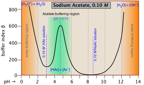
This buffer index plot for a 0.10 M solution of sodium acetate is typical, and confirms that buffering is most efficient within about ±1 pH unit of pKa.
But what about the even greater buffering that apparently occurs at the two extremes of pH (orange shading)? This is due to the buffering associated with the water itself, and will be seen in all aqueous buffer solutions.
Pure water is buffered by the H3O+/H2O conjugate pair at very low pH, and by
H2O/OH- at high pH. This is easily understood if you think about adding some strong acid acid to pure water; even one drop of HCl will send the pH shooting down toward 0. If you continue adding acid, the pH will not drop significantly below 0, because there won't be enough free water molecules remaining to hydrate the HCl to produce H3O+ ions — thus the solution is strongly buffered.
Note that if we were to subtract the effect of the NaAc buffering from the above plot, the remaining plot for water itself would exhibit a minimum at pH 7, where both [H3O+] and [OH–] share a common minimum value.
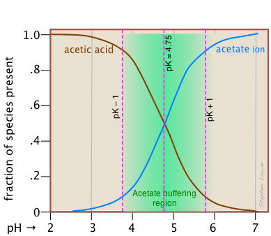
This alternative view shows how the distribution fractions of HAc and Ac– relate to the effective buffering range of this conjugate pair, which is conventionally defined as ±1 pH unit of the pKa.
Buffer capacity
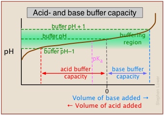 As we mentioned in the sidebar above, the term buffer capacity is an alternative means of expressing the ability of a buffer system to absorb the addition of strong acid or base without causing the pH to deviate by more than one unit from that of the pure buffer.
In this example, the buffer capacities for addition of acid and base will differ because the buffer pH has been adjusted to a value that differs from its pKa.
The importance of buffer concentration
Buffer systems must be appreciably more concentrated than the concentrations of strong acid or base they are required to absorb while still remaining within the desired pH range. Once the added acid or base has consumed most of one or other of the conjugate species comprising the buffer, the pH will no longer be stabilized. And of course, very small buffer concentrations will approach the pH of pure water.
 These plots are often referred to as Sillén plots. Lars Gunnar Sillén (1916-1970) was a Swedish chemist and textbook author who studied the distribution of ionic species in aqueous solutions and especially in the oceans.
Because the concentrations of conjugate species can vary over many orders of magnitude, it is far more useful to express them on a logarithmic scale. Since pH is already logarithmic, one can obtain a "bird's-eye view" of an acid-base system in a compact log-log plot.
Even better, these plots are easily constructed without any calculations or arithmetic — or even any graph paper — any scrap paper, even the back of an envelope, will be sufficient. A ruler or other straightedge will, however, give more accurate results.
In addition, you can use these plots to estimate the pH of a solution of a monoprotic or polyprotic acid or base without contending with quadratic or higher-order equations — or doing any arithmetic at all! The results will not be as precise as you would get from a proper numerical solution, but given the uncertainties of how equilibrium constants are affected by the presence of other ions in the solution, this is rarely a problem.
But aside from these advantages, the use of log-C vs pH plots will afford you an insight into the chemistry of acid-base systems that cannot be obtained simply by doing numerical calculations.
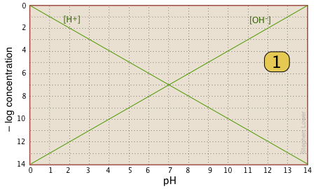
The basic form of the plot, and the starting point for any use of such plots, looks like this:
![]()
If you examine this plot carefully, you will see that it is nothing more than a definition of pH and pOH, as well as a definition of a neutral solution at pH 7. Notice, for example, that when the pH is 4.0,
[H+] = 10–4 M and
[OH–] = 10–10 M.
A simple example: acetic acid solution
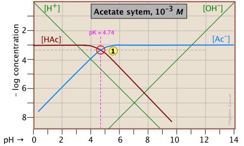 Here is a log C plot for a 10–3 M solution of acetic acid ("HAc") in water. Although it may look a bit complicated at first, it is really very simple. The heavy maroon line on the left plots the concentration of the acid HAc as a function of pH. The blue line on the right shows how the concentration of the base Ac– depends on pH. The horizontal parts of these lines are aligned with "3" on the –log-C axis, corresponding to the 10–3 M nominal concentration (Ca).
How do we know the shapes and placement of the plots for the concentrations of acetic acid [HAc] and the acetate ion [Ac–] ?
- At very low pH, virtually all of the acetate system will be in its acid form
(that is, [HAc] = 10–3), and similarly, at high pH, the base form [Ac–] = 10–3 M. - When pH = pKa, the concentrations of the conjugate species are identical, as indicated by the crossing of the lines representing the two concentrations. These concentrations will be half of the total concentration given by Ca, so [HAc] = [Ac–] = ½Ca = 0.5E–3 M. Where does this go on the log-C axis? Well, the logarithm of 0.5 is –0.3 (a useful fact to remember!), so the crossing point at
 is displaced by 0.3 of a log-C unit below the –3 level on the y-axis.
 - Because point defines both the pKa and concentration of a particular acid-base system, it is known as the system point.
- What about the slopes of the plots when they bend down? It turns out that these slopes are +1 for
[Ac–] and –1 for [HAc]. Since the slopes of the lines for [H+] and [OH–] are ±1, we can use these as guidelines; just make the plots of [Ac–] and [HA] parallel to them. - The curved portions of the plot that joins the the horizontal and diagonal parts on either side of the system point can be drawn freehand without undue error; logarithmic plots are very forgiving!
Although both of these concentrations will of course vary with the pH, their deviations from 10–3 M are too small to reveal themselves on a logarithmic plot until the pH approaches the pKa.
Estimating the pH
Of special interest in acid-base chemistry are the pH values of a solution of an acid and of its conjugate base in pure water; as you know, these correspond to the beginning and equivalence points in the titration of an acid with a strong base. Continuing with the example of the acetic acid system, we show below another plot that is just like the one above, but with a few more lines and numbers added.
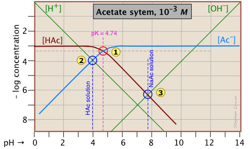 pH of acetic acid in pure water. Suppose you would like to find the pH of a 0.001 M solution of acetic acid in pure water. From the equation
HAc + H2O → H3O+ + Ac–(2-1)
we know that equal numbers of moles of hydronium and acetate ions will be formed, so the concentrations of these species should be about the same:
[H+] ≈ [Ac–](2-2)
will hold. The equivalence of these two concentrations corresponds to the point labeled ![]() on the logC-pH plot; this occurs at a pH of about 4, and this is the pH of a 0.001 M solution of acetic acid in pure water.
on the logC-pH plot; this occurs at a pH of about 4, and this is the pH of a 0.001 M solution of acetic acid in pure water.
pH of sodium acetate in pure water. A 0.001 M solution of NaAc in water corresponds to the composition of a solution of acetic acid that has been titrated to its equivalence point with sodium hydroxide. The acetate ion, being the conjugate base of a weak acid, will undergo hydrolysis according to
Ac– + H2O → HAc + OH– (2-3)
which establishes the approximate relation
[HAc] ≈ [OH–](2-4)
This condition occurs where the right sloping part of the line representing [HAc] intersects the [OH–] line at ![]() in the plot above. As you would expect for a solution of the conjugate base of a weak acid, this corresponds to an alkaline solution, in this case, at about pH = 7.8.
in the plot above. As you would expect for a solution of the conjugate base of a weak acid, this corresponds to an alkaline solution, in this case, at about pH = 7.8.
You will have to admit that estimating a pH in this way is far more painless than an ordinary numerical calculation would be!
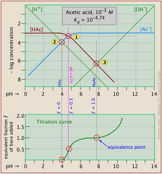
It is interesting to show the Sillén plot for a weak acid system with its titration curve, both on the same pH scale.
In this example, the titration plot has been turned on its side and reversed in order to illustrate the correspondence of its ƒ=0 (initial), ƒ=0.5 and ƒ=1 (equivalence) points with the corresponding points on the upper plot.
Ammonia - a weak base
Ammonia, unlike most gases, is extremely soluble in water. Solutions of NH3 in water are properly known as aqueous ammonia, NH3(aq); the name "ammonium hydroxide" is still often used, even though there is no evidence to suggest that a species NH4OH exists.
Ammonia is the conjugate base of the ammonium ion NH4+. The fact that ammonia is a base has no special significance insofar as the construction and interpretation of the log-C vs pH diagram is concerned; such diagrams always refer to conjugate acid-base systems, rather than to individual acids and bases.
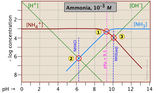 Thus the system point
 ![]() defines the NH4+/NH3 pair (pKa 9.3) at 25°C and a total concentration
defines the NH4+/NH3 pair (pKa 9.3) at 25°C and a total concentration
CT = Ca + Cb = 0.0010 M.
In order to estimate the pH of a solution of ammonia in pure water, we make use of the charge balance requirement (known as the proton condition)
[NH4+] + [H+] = [OH–](2-5)
which we simplify by assuming that, because NH4+ is a weak acid, [NH4+] >> [H+] and we can drop the [H+] term; thus the approximation
[NH4+] ≈ [OH–](2-6)
which corresponds to the crossing point ![]() and a pH of 10.0.
and a pH of 10.0.
Similarly, at the crossing point ![]() , [NH3] ≈ [H+]. This comes from the proton condition [NH3] + [H+] – [OH–] = 0 by dropping the [OH–] term on the assumption that its value is negligible compared to [H+].
, [NH3] ≈ [H+]. This comes from the proton condition [NH3] + [H+] – [OH–] = 0 by dropping the [OH–] term on the assumption that its value is negligible compared to [H+].
You will have noticed that we referred to Eq ?? as the "proton condition". Sorry to sneak it in without warning, but we hope that having piqued your curiosity, you might take the time to look at the following discussion of this important tool for estimating the pH of a solution of a pure acid, base, or a salt.
Mass- and charge balance, and the proton condition
In any aqueous solution of an acid or base, certain conservation conditions are strictly observed. Together with concentration and the Ka or Kb , these put certain constraints on the system that determine the state of the system.
The most fundamental of these are conservation of mass and of electric charge, which of course apply to chemical changes of all kinds. We commonly express these as mass balance and charge balance, respectively. (The latter of these is sometimes referred to as the electroneutrality condition.)
Using the above example of the ammonium system as an illustration of this, we are interested in two particular instances of practical importance: what conditions apply to solutions made by dissolving a) pure ammonia,
or b) ammonium chloride, in water?
- Mass balances
- CT, NH3 = [NH3] + [NH4+] = 10–2 M
- CT, Ac = [HAc] + [Ac–] = 10–2 M
- Charge balances
- NH3: [H+] + [NH4+] = [OH–]
- NaAc: [Na+] + [H+] = [Ac–] + [OH–]
OK so far? That's really all we need, but it's usually more convenient to combine these with mass balances on the protons alone, so that we have a single equation for each of the two solutions. The resulting equations are known as the proton conditions for the two solutions.
In order to avoid a lot of algebra, there is a simple short-cut for writing a proton condition equation:
- Identify the substance you are starting with — the pure acid, base, or salt, and also H2O itself, that make up the solution whose pH you wish to know at the concentration for which the log C-pH chart is drawn. we call this the proton reference level (if that appellation scares you, it is sometimes referred to as the "basis substance".)
- On the left side of the proton condition, write concentration expressions for all species that possess protons in excess of the reference level.
- On the right side, write concentrations of all species that possess fewer protons the reference level.
Let's try it for our ammonia system.
Solution of NH3 in water:
The proton reference level (PRL) is defined by NH3(aq) and H2O.
Proton condition: [H3O+] + [NH4+] = [OH–]
(Notice that the substances that define the PRL (in case, H2O and NH3) never appear in the proton condition equation.)
Solution of NH4Cl (or of any other strong-anion ammonium salt) in water:
The PRL is defined by NH4+ and H2O.
Proton condition: [H3O+] = [NH3] + [OH–]
(The chloride ion has nothing to do with protons, so it does not appear here.)
This proton condition stuff seems awfully complicated: why do we bother?
Good question: the answer is that what seems complicated at first sometimes turns out to be simpler and easier to understand than any alternative.
Think of it this way: acid-base reactions involve the transfer of protons: some protons jump up to higher proton-free energy levels
(e.g., NH3 + H2O → NH4+ + OH–), others drop down to proton-vacant levels (H3O+ → NH3 → H2O + NH4+). But no matter what happens, the total number of "available" protons (that is, all "dissociable" protons, including those in
H3O+) must be conserved — thus the "mass balance on protons".
So let's look again at the log C - pH plot for the ammonium system, which we reproduce here for your convenience:
Consider first the solution of ammonium chloride, whose proton condition is given by [H3O+] = [NH3] + [OH–]. We know that NH4Cl, being the salt of a weak base and a strong acid, will give a solution that is slightly acidic. In such a solution, [OH–] will be quite small so that we can neglect it without too much error. We can then write the proton condition as [H+] ≈ [NH3]. On the plot above, this corresponds to point ![]() where the lines representing these quantities cross. At this pH of around 6.2, [OH–] is about two orders of magnitude smaller than [NH3], so we are justified in dropping it.
where the lines representing these quantities cross. At this pH of around 6.2, [OH–] is about two orders of magnitude smaller than [NH3], so we are justified in dropping it.
Similarly, for a solution of ammonia in water, the proton condition
[H3O+] + [NH4+] = [OH–] that we worked out above can be simplified to
[NH4+] ≈ [OH–] (point ![]() ) with hardly any error at all, since [H+] is here about six orders of magnitude smaller than [NH4+].
) with hardly any error at all, since [H+] is here about six orders of magnitude smaller than [NH4+].
In our discussion of the plot for the acetic acid system, we arrived at the proton conditions [H+] ≈ [Ac–] (for HAc in water) and [H+] ≈ [OH–] (for NaAc) by simply using the stoichiometries of the reactions. This can work in the simplest systems, but not in the more complicated ones involving polyprotic systems. In general, it is far safer to write out the complete proton condition in order to judge what concentrations, if any, can be dropped.
Ammonium acetate solution: solution of a salt
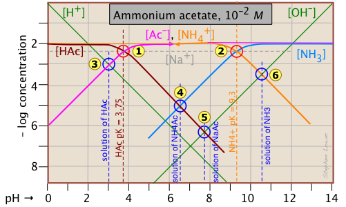 Having looked at the Sillén diagrams for acetic acid and ammonia, let's examine the log C-pH plot for this salt of acetic acid and ammonia.
You will recall that we dealt with solutions of the salts sodium acetate and ammonium chloride in the two examples described above. What is different here is that both components of the salt CH3COONH4 ("NH4Ac") are "weak" in the sense that their conjugate species NH3 and HAc are also present in significant quantities. This means that we are really dealing with two acid-base systems — the ones shown previously — on the same plot.
Each system retains its own system point, ![]() for the acetate system and
for the acetate system and ![]() for the ammonium system.
for the ammonium system.
Note that the two plots previously shown were for 10–3 M solutions, so the non-system points for this more concentrated solution occur at different pH values. The pH's of 10–2 M solutions of HAc ![]() , NaAc
, NaAc ![]() , and NH3
, and NH3 ![]() are located by using the same proton conditions as before.
are located by using the same proton conditions as before.
The only new thing here is the point ![]() , which corresponds to the ammonium acetate solution in which we are interested. The proton condition for this solution is [H+] + [HAc] = [NH3(aq)] + [OH–]. Inspection of the plot reveals that [H+] << [HAc] and [OH–] << [NH3(aq)], so the proton condition can be simplified to [HAc] ≈ [NH3(aq)], corresponding to the intersection of these two lines at
, which corresponds to the ammonium acetate solution in which we are interested. The proton condition for this solution is [H+] + [HAc] = [NH3(aq)] + [OH–]. Inspection of the plot reveals that [H+] << [HAc] and [OH–] << [NH3(aq)], so the proton condition can be simplified to [HAc] ≈ [NH3(aq)], corresponding to the intersection of these two lines at ![]() .
.
Polyprotic systems
Now that you are able to find your way around log C-pH plots that encompass two acid-base systems, the polyprotic systems that we describe below should be no trouble at all.
The carbonate system
A thorough understanding of the carbonic acid-carbonate system is essential for understanding the chemistry of natural waters and the biochemistry of respiration in humans and other animals.
There are two special things about this system that you need to know:
- A solution of carbon dioxide in water is mostly in the form of hydrated CO2, CO2(aq). But a small fraction of dissolved CO2 reacts with water to form carbonic acid, H2CO3. Because this acid cannot be isolated, common practice is to add an asterisk to the formula to designate the "total" CO2 concentration
[CO2 + H2CO3]: thus H2CO3*. - Because CO2 is a gas, solutions containing carbonate species of all kinds can equilibrate with the atmosphere, which normally contains small quantities of CO2. This means that a solution of sodium bicarbonate that is open to the atmosphere can lose CO2 to the atmosphere at low pH, and absorb it at high pH. A system of this kind is said to be open. Alternatively, a system can be closed to exchange with the atmosphere. Sillén plots for open and closed carbonate systems have very different appearances.
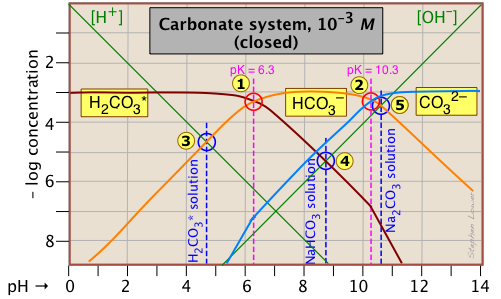 This Sillén plot for the
H2CO3* closed system is typical of other diprotic acid systems in that there are three conjugate species and two system points. The 10–3 M concentration plotted here is typical of what is found in groundwaters that are in contact with carbonate-containing sediments.
The pH of a 10–3 M solution of CO2, NaHCO3 and Na2CO3 are indicted by the blue annotations.
| solute, (reference level) | proton condition | approximation |
|---|---|---|
| carbon dioxide (H2CO3*) | [H+] = [HCO3–] + 2[CO32–] + [OH–] | [H+] ≈ [HCO3–] |
| sodium bicarbonate (NaHCO3) | [H+] + [H2CO3] = [CO32–] + [OH–] | [H2CO3] ≈ [OH–] |
| sodium carbonate (Na2CO3) | [H+] + 2[H2CO3*] + [HCO3–] = [OH–] | [HCO3–] ≈ [OH–] |
You should take a few moments to verify the approximations in the rightmost column.
Notice the factors of 2 that multiply some of the concentrations. For example, the "2[CO32–]" term in the first line of the table means that the CO32– species is two steps away from the proton reference level H2CO3*, so it would take two hydrogen ions to balance a single carbonate ion.
Another new feature introduced here is the doubling of the slopes of the lines representing [H2CO3*] and [CO32–] where they cross the pH values corresponding to the Kas that are one step removed from their own system points ![]() and
and ![]() near –log C = 7.
near –log C = 7.
The phosphate system
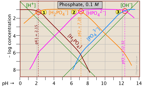 This triprotic system is widely used to prepare buffer solutions in biochemical applications. In its fundamental form, there is nothing new here, other than an additional system point
 ![]() corresponding to the pKa of H2PO4–.
corresponding to the pKa of H2PO4–.
The pH of a 10–3 M solutions of H3PO4, NaH2PO4, Na2HPO4 and Na3PO4can be estimated by setting up the proton conditions as follows. Unfortunately, these estimates become a bit more complicated owing to the proximity of the three system points. But it's far easier than doing a numerical solution which requires solving a firth-degree polynomial!
| solute, (reference level) | proton condition | approximation |
|---|---|---|
| phosphoric acid (H3PO4) | [H+] = [H2PO4–] + 2[HPO42–] + 3[PO43–] + [OH–] | [H+] ≈ [H2PO4–] |
| sodium dihydrogen phosphate (NaH2PO4) | [H+] + [H3PO4] = [HPO42–] + 2[PO43–] + [OH–] | [H+] + [H3PO4] ≈ [HPO42–] |
disodium hydrogen phosphate (Na2HPO4) |
[H+] + 2[H2PO4–] + [H2PO4–] = 3[PO43–] + [OH–] | [H3PO4-] = [PO43–] + [OH–] |
| trisodium phosphate (Na3PO4) | [H+] + 3[H3PO4] +2 [H2PO4–] + [HPO42–] = [OH–] | [HPO42–] ≈ [OH–] |
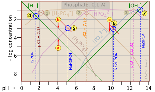 Because the phosphate plot is rather crowded, we show here a modified one in which the details of the pH estimates for the solutions of H3PO4 and its salts are emphasized.
Estimation of the pH of 10–3 M solutions of phosphoric acid ![]() and trisodium phosphate
and trisodium phosphate ![]() , based on the approximations in the above table are straightforward.
, based on the approximations in the above table are straightforward.
Those for NaH2PO4 ![]() and Na2HPO4
and Na2HPO4 ![]() , however, are complicated by the presence of two concentration terms on the right side of the respective proton condition approximations.
, however, are complicated by the presence of two concentration terms on the right side of the respective proton condition approximations.
Unless you are in an advanced course, you may wish to skip the following details. The important thing to know is that graphical estimates of these more problematic systems are fundamentally possible.
Thus for sodium dihydrogen phosphate, if we were to follow the pattern of the other systems, the approximation at the crossing point would be
[H+] = [HPO42–], corresponding to point ![]() . But inspection of the plot shows that at that pH (4.0), the concentration of H3PO4 is ten times greater than that of H+ (point
. But inspection of the plot shows that at that pH (4.0), the concentration of H3PO4 is ten times greater than that of H+ (point ![]() ). A rough estimate of the pH can be made by constructing a line (shown in red) that is parallel to those for H3PO4 and H+, but is raised up by a factor of 10. This results in the new crossing point
). A rough estimate of the pH can be made by constructing a line (shown in red) that is parallel to those for H3PO4 and H+, but is raised up by a factor of 10. This results in the new crossing point ![]() .
.
Similarly, the pH of a disodium hydrogen phosphate solution does not correspond to the crossing point ![]() because of the significant value of [HPO43–] at this pH. Again, we construct a line above this crossing point that predicts a pH corresponding to point
because of the significant value of [HPO43–] at this pH. Again, we construct a line above this crossing point that predicts a pH corresponding to point ![]() .
.
Although these stratagems may seem rather crude, it should be noted that the uncertainties associated with them tend to be minimized on a logarithmic plot. In addition, it should be borne in mind that in a solution as concentrated as 0.1M, the pKa values found in tables are not applicable. The alternative of solving for the pH algebraically, taking into consideration activity coefficients for the high ionic concentrations, is rarely worth the effort.
This is more advanced material that can be skipped by first-year students.
The relation between the pH of a solution and the concentrations of weak acids and their conjugate species is algebraically rather complicated. But over most of the pH range, simplifying assumptions can be made that, when expressed in logarithmic form, plot as straight lines having integral slopes of 0, ±1, ±2, etc.
It is only within the narrow pH range near the pKa that these simplifying assumptions break down, but on a logarithmic plot, one can draw a smooth curve that covers this range without introducing significant error.
Here is your basic stationery — a plot showing the two ions always present in any aqueous solution. In practice, you can usually cut off the bottom part where concentrations smaller than |
 |
For any given acid-base system, you need to know the pKa and nominal concentration CT. Find the point at which these two lines intersect. |
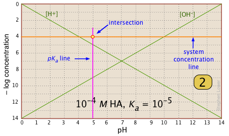 |
Locate and mark the system point on the pKa line. It will be 0.3 of a log-C unit below the concentration line. This is where [HA] |
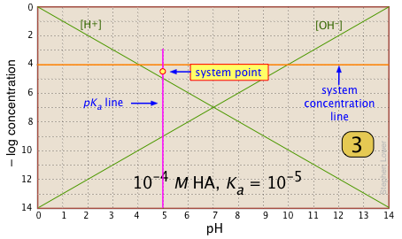 |
For pH < pKa, [HA] plots as a line through the system point with slope = 0. For pH > pKa, the line assumes a slope of –1. Use the [H+] and |
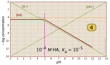 |
| In the pH interval of ±pKa, the slope changes from 0 to +1. You can approximate this with a sloped line as shown, or "prettify" it with a smooth curve. | 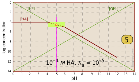 |
| Finally, draw the lines for the conjugate form [A–], using slopes +1 and 0. | 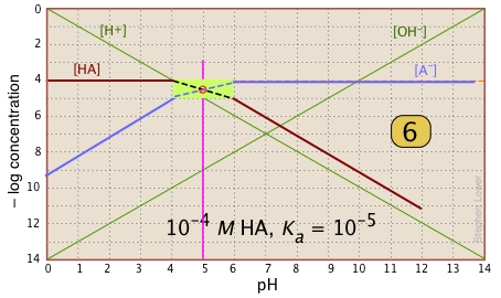 |
What's all this good for?
Suppose you have a solution of NaA whose pH is 8. Estimate the concentration of the acid HA in the solution.
All you need do is look at the plot. The [HA] line crosses the line marking this pH at – log C = 6, or [HA] = 10–6. This quantity too small to significantly reduce [A–], which remains at approximately CT = 10–6 M.
Boundless outlines on buffer solutions. These summarize the main points and problem examples as presented in major textbooks. They are an excellent aid for pre-exam review. Chemistry: The Central Science (8 subtopics)
A collection of practice exercises (with solutions) on buffers and titrations from Bryn Mawr College.
The Henderson-Hasselbalch equation: its history and limitations - Henry N. Po and N.M. Senoza, J.Chem. Ed. 78 (11) 2001 (1499-1503)
A detailed treatment of log-C vs pH diagrams can be found in the book Acid-base diagrams by Kahlert and Schotz. It is available online in some college libraries.
Make sure you thoroughly understand the following essential concepts that have been presented above.
- State the values of Ca and Cb after a weak monoprotic acid or base has been partially neutralized with strong base or acid. (Problem Example 1)
- Define the ionization fraction, and calculate the percent ionization, of a Ca M solution of a weak monoprotic acid.
- Sketch out a rough plot showing the distribution of conjugate species in a solution of a weak acid having a given value of Ka.
- Define a buffer solution, and explain how it works.
- Calculate the approximate pH of a solution of a weak monoprotic acid having a given pKa that has been partially neutralized by addition of a strong base.
- Specify how to make a given volume of a buffer solution having a certain pH, starting with a weak acid and sodium hydroxide. (Problem Example 3)
- Define the buffer index, and explain its significance and the conditions under which its value is maximized.
- Sketch out a –log C vs pH (Sillén) plot for a weak monoprotic acid/base system having a given nominal concentration and pKa, and use it to estimate the pH of the solution.

© 2004-2014 by Stephen Lower - last modified 2018-12-28
The Chem1 Virtual Textbook home page is at http://www.chem1.com/acad/virtualtextbook.html

This work is licensed under a
Creative Commons Attribution-Share Alike 3.0 License.