Drawing conclusions from data

In the previous section of this unit we examined two very simple sets of data:

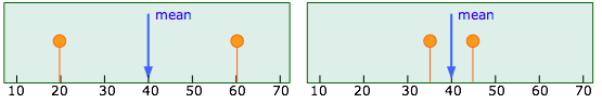
Each of these sets has the same mean value of 40, but the "quality" of the set shown on the right is greater because the data points are less scattered; the precision of the result is greater. The quantitative measure of this precision is given by the standard deviation

whose value works out to 28 and 7 for the two sets illustrated above. A data set containing only two values is far too small for a proper statistical analysis— you would not want to judge the average mercury content of canned tuna on the basis of only two samples, for instance. Suppose, then, for purposes of illustration, that we have accumulated many more data points but the standard deviations of the two sets remain at 28 and 7 as before. What conclusions can we draw about how close the mean value of 40 is likely to come to the "true value" (the population mean μ) in each case?

Although we cannot ordinarily know the value of μ, we can assign to each data point x_i a quantity (x_i – x_m) which we call the deviation from the [population] mean, an index of how far each data point differs from the elusive “true value”. We now divide this deviation from the mean by the standard deviation of the entire data set:

If we plot the values of z that correspond to each data point, we obtain the following curves for the two data sets we are using as examples:

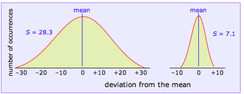
We won’t attempt to prove it here, but the mathematical properties of a Gaussian curve are such that its shape depends on the scale of units along the x-axis and on the standard deviation of the corresponding data set. In other words, if we know the standard deviation of a data set, we can construct a plot of z  that shows how the measurements would be distributed

• if the number of observations is very large
• if the different values are due only to random error

An important corollary to the second condition is that if the data points do not approximate the shape of this curve, then it is likely that the sample is not representative, or that some complicating factor is involved. The latter often happens when a teacher plots a set of student exam scores, and gets a curve having two peaks instead of one— representing perhaps the two sub-populations of students who devote their time to studying and partying.

This little gem was devised by the statistician W.J. Youdan and appears in The visual display of quantitative information, an engaging book by Edward R. Tufte (Graphics Press, Cheshire CT, 1983).

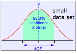
Clearly, the sharper and more narrow the standard error curve for a set of measurement, the more likely it will be that any single observed value approximates the true value we are trying to find. Because the shape of the curve is determined by S, we can make quantitative predictions about the reliability of our data from its standard deviation. In particular, if we plot z as a function of the number of standard deviations from the mean (rather than as the number of absolute deviations from the mean as was done above), the shape of the curve depends only on the value of S. That is, the dependence on the particular units of measurement is removed.

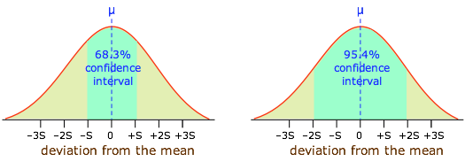
Moreover, it can be shown that if all measurement error is truly random, 68.3 percent (about two-thirds) of the data points will fall within one standard deviation of the population mean, while 95.4 percent of the observations will differ from the population mean by no more than two standard deviations. This is extremely important, because it allows us to express the reliability of a measurement quantitatively, in terms of confidence intervals.

This is as close to “the truth” as we can get in scientific measurements.

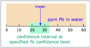Note carefully: Confidence interval (CI) and confidence level (CL) are not the same!

A given CI (denoted by the shaded range of 18-33 ppm in the diagram) is always defined in relation to some particular CL; specifying the first without the second is meaningless. If the CI illustrated here is at the 90% CL, then a CI for a higher CL would be wider, while that for a smaller CL would encompass a smaller range of values.

The units of CI are those of the measurement (e.g., ppm); CL itself is usually expressed in percent.

The more measurements we make, the more likely will their average value approximate the true value. The width of the confidence interval (expressed in the actual units of measurement) is directly proportional to the standard deviation S  and to the value of z (both of these terms are defined above). The confidence interval of a single measurement in terms these quantities and of the observed sample mean is given by:

CI = x_m + z S

If n replicate measurements are made, the confidence interval becomes smaller:

This relation is often used “in reverse”, that is, to determine how many replicate measurements n  must be carried out in order to obtain a value within a desired confidence interval.

As we pointed out above, any relation involving the quantity z (which the standard error curve is a plot of) is of limited use unless we have some idea of the value of the population mean μ. If we make a very large number of measurements (100 to 1000, for example), then we can expect that our observed sample mean approximates μ quite closely, so there is no difficulty.

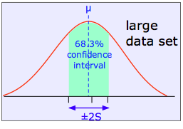
The shaded area in each plot shows the fraction of measurements that fall within two standard deviations (2S) of the "true" value (that is, the population mean μ). It is evident that the width of the confidence interval diminishes as the number of measurements becomes greater. This is basically a result of the fact that relatively large random errors tend to be less common than smaller ones, and are therefore less likely to cancel out if only a small number of measurements is made.

OK, so larger data sets are better than small ones. But what if it is simply not practical to measure the mercury content of 10,000 cans of tuna? Or if you were carrying out a forensic examination of a tiny chip of paint, you might have only enough sample (or enough time) to do two or three replicate analyses. There are two common ways of dealing with such a difficulty.

One way of getting around this is to use pooled data; that is, to rely on similar prior determinations, carried out on other comparable samples, to arrive at a standard deviation that is representative of this particular type of determination.

The other common way of dealing with small numbers of replicate measurements is to look up, in a table, a quantity t, whose value depends on the number of measurements and on the desired confidence level. For example, for a confidence level of 95%, t would be 4.3 for three samples and 2.8 for five. The magnitude of the confidence interval is then given by

CI = ± t S

This procedure is not black magic, but is based on a careful analysis of the way that the Gaussian curve becomes distorted as the number of samples diminishes.

Once we have obtained enough information on a given sample to evaluate parameters such as means and standard deviations, we are often faced with the necessity of comparing that sample (or the population it represents) with another sample or with some kind of a standard. The following sections paraphrase some of the typical questions that can be decided by statistical tests based on the quantities we have defined above. It is important to understand, however, that because we are treating the questions statistically, we can only answer them in terms of statistics— that is, to a given confidence level.

The usual approach is to begin by assuming that the answer to any of the questions given below is “no” (this is called the null hypothesis), and then use the appropriate statistical test to judge the validity of this hypothesis to the desired confidence level.

Because our purpose here is to show you what can be done rather than how to do it, the following sections do not present formulas or example calculations, which are covered in most textbooks on analytical chemistry. You should concentrate here on trying to understand why questions of this kind are of importance. For more detail, see Statistics at Square One. This online reference has good descriptions of the t-test and of the other applications described below./p>

“Should I throw this measurement out?”

That is, is it likely that something other than ordinary indeterminate error is responsible for this suspiciously different result? Anyone who collects data of almost any kind will occasionally be faced with this question. Very often, ordinary common sense will be sufficient, but if you need some help, two statistical tests, called the Q test and the T test, are widely employed for this purpose.

We won’t describe them here, but both tests involve computing a quantity (Q or T) for a particular result by means of a simple formula, and then consulting a table to determine the likelyhood that the value being questioned is a member of the population represented by the other values in the data set.

A good Q test tutorial (U of Toronto)  

“Does this method yield reliable results?"

This must always be asked when trying a new method for the first time; it is essentially a matter of testing for determinate error. The answer can only be had by running the same procedure on a sample whose composition is known. The deviation of the mean value of the “known” x_m from its true value μ is used to compute a Student's t for the desired confidence level. You then apply this value of t to the measurements on your unknown samples.

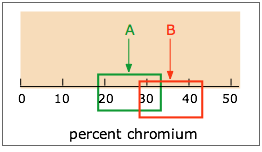
“Are these two samples identical?”

You wish to compare the means x_m1 and x_m2 from two sets of measurements in order to assess whether their difference could be due to indeterminate error. Suppose, for example, that you are comparing the percent of chromium in a sample of paint removed from a car's fender with a sample found on the clothing of a hit-and-run victim. You run replicate analyses on both samples, and obtain different mean values, but the confidence intervals overlap. What are the chances that the two samples are in fact identical, and that the difference in the means is due solely to indeterminate error?

A fairly simple formula, using Student’s t, the standard deviation, and the numbers of replicate measurements made on both samples, provides an answer to this question, but only to a specified confidence level. If this is a forensic investigation that you will be presenting in court, be prepared to have your testimony demolished by the opposing lawyer if the CL is less than 99%.

“What is the smallest quantity I can detect?”

This is just a variant of the preceding question. Estimation of the detection limit of a substance by a given method begins with a set of measurements on a blank, that is, a sample in which the substance of question is assumed to be absent, but is otherwise as similar as possible to the actual samples to be tested. We then ask if any difference between the mean of the blank measurements and of the sample replicates can be attributed to indeterminate error at a given confidence level.

For example, a question that arises at every world Olympics event, is what is the minimum level of a drug metabolite that can be detected in an athlete's urine? Many sensitive methods are subject to random errors that can lead to a non-zero result even in a sample known to be entirely free of what is being tested for. So how far from "zero" must the mean value of a test be in order to be certain that the drug was present in a particular sample? A similar question comes up very frequently in environmental pollution studies.

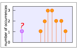
Throwing away “wrong” answers.

It occasionally happens that a few data values are so greatly separated from the rest that they cannot reasonably be regarded as representative. If these “outliers” clearly fall outside the range of reasonable statistical error, they can usually be disregarded as likely due to instrumental malfunctions or external interferences such as mechanical jolts or electrical fluctuations.

Some care must be exercised when data is thrown away however; There have been a number of well-documented cases in which investigators who had certain anticipations about the outcome of their experiments were able to bring these expectations about by removing conflcting results from the data set on the grounds that these particular data “had to be wrong”

Beware of too-small samples

The probability of ten successive flips of a coin yielding 8 heads is given by

... indicating that it is not very likely, but can be expected to happen about eight times in a thousand runs. But there is no law of nature that says it cannot happen on your first run, so it would clearly be foolish to cry “Eureka” and stop the experiment after one— or even a few tries. Or to forget about the runs that did not turn up 8 heads!

Perils of dubious "correlations"

The fact that two sets of statistics show the same trend does not prove they are connected, even in cases where a logical correlation could be argued. Thus it has been suggested that according to the two plots below, "In relative terms, the global temperature seems to be tracking the average global GDP quite nicely over the last 70 years."

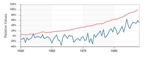
(Data from the former EconStats Web site)

Perils of a too-low confidence level

The difference between confidence levels of 90% and 95% may not seem like much, but getting it wrong can transform science into junk science — a not-unknown practice by special interests intent on manipulating science to influence public policy; see the excellent 2008 book by David Michaels "Doubt is Their Product: How Industry's Assult on Science Threatens Your Health".