Reliability of a measurement
Making sense of all those numbers
In this day of pervasive media, we are continually being bombarded with data of all kinds— public opinion polls, advertising hype, government reports and statements by politicians. Very frequently, the purveyors of this information are hoping to “sell” us on a product, an idea, or a way of thinking about someone or something, and in doing so, they are all too often willing to take advantage of the average person’s inability to make informed judgements about the reliability of the data, especially when it is presented in a particular context (popularly known as “spin”.)
In Science, we do not have this option: we collect data and make measurements in order to get closer to whatever “truth” we are seeking, but it's not really "science" until others can have confidence in the reliability of our measurements.
The kinds of measurements we will deal with here are those in which a number of separate observations are made on individual samples taken from a larger population.
Population, when used in a statistical context, does not necessarily refer to people, but rather to the set of all members of the group of objects under consideration.
For example, you might wish to determine the amount of nicotine in a manufacturering run of one million cigarettes. Because no two cigarettes are likely to be exactly identical, and even if they were, random error would cause each analysis to yield a different result, the best you can do would be to test a representative sample of, say, twenty to one hundred cigarettes. You take the average (mean) of these values, and are then faced with the need to estimate how closely this sample mean is likely to approximate the population mean. The latter is the “true value” we can never know; what we can do, however, is make a reasonable estimate of the likelyhood that the sample mean does not differ from the population mean by more than a certain amount.
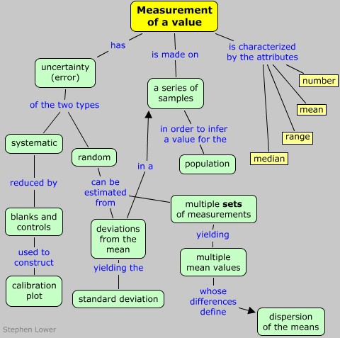
The attributes we can assign to an individual set of measurements of some quantity x within a population are listed below. It is important that you learn the meaning of these terms:
- Number of measurements
- This quantity is usually represented by n.
- Mean
- The mean value xm (commonly known as the average), defined as
- Median
- The median value, which we will not deal with in this brief presentation, is essentially the one in the middle of the list resulting from writing the individual values in order of increasing or decreasing magnitude.

Don't let this notation scare you!
It just means that you add up all the values
and divide by the number of values,
just like you did in Grade 6.
"Dispersion" means "spread-outedness". If you make a few measurements and average them, you get a certain value for the mean. But if you make another set of measurements, the mean of these will likely be different. The greater the difference between the means, the greater is their dispersion.
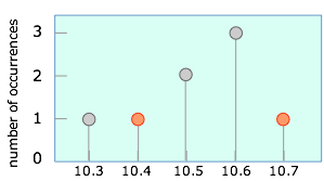 Suppose that instead of taking the five measurements as in the above example, we had made only two observations which, by chance, yielded the values that are highlighted here. This would result in a sample mean of 10.45. Of course, any number of other pairs of values could equally well have been observed, including multiple occurances of any single value.
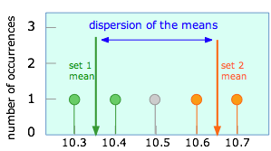 Shown at the left are the results of two possible pairs of observations, each giving rise to its own sample mean. Assuming that all observations are subject only to random error, it is easy to see that successive pairs of experiments could yield many other sample means. The range of possible sample means is known as the dispersion of the mean.
It is clear that neither of these two sample means will likely correspond to the population mean, whose value we are really trying to discover. It is a fundamental principle of statistics, however, that the more observations we make in order to obtain a sample mean, the smaller will be the dispersion of the sample means that result from repeated sets of the same number of observations. (This is important; please read the preceding sentence at least three times to make sure you understand it!)
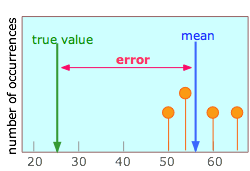
How the disperson of the mean depends on the number of observations
 The difference between the sample mean (blue) and the population mean (the "true value", green) is the error of the measurement. It is clear that this error diminishes as the number of observations is made larger.
What is stated above is just another way of saying what you probably already know: larger samples produce more reliable results. This is the same principle that tells us that flipping a coin 100 times will be more likely to yield a 50:50 ratio of heads to tails than will be found if only ten flips (observations) are made.
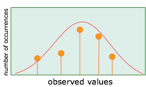
The reason for this inverse relation between the sample size and the dispersion of the mean is that if the factors giving rise to the different observed values are truly random, then the more samples we observe, the more likely will these errors cancel out. It turns out that if the errors are truly random, then as you plot the number of occurences of each value, the results begin to trace out a very special kind of curve.
 The significance of this is much greater than you might at first think, because the gaussian curve has special mathematical properties that we can exploit, through the methods of statistics, to obtain some very useful information about the reliability of our data. This will be the major topic of the next lesson in this set.
For now, however, we need to establish some important principles regarding measurement error.
The scatter in measured results that we have been discussing arises from random variations in the myriad of events that affect the observed value, and over which the experimenter has no or only limited control. If we are trying to determine the properties of a collection of objects (nicotine content of cigarettes or lifetimes of lamp bulbs), then random variations between individual members of the population are an ever-present factor. This type of error is called random or indeterminate error, and it is the only kind we can deal with directly by means of statistics.
 There is, however, another type of error that can afflict the measuring process. It is known as systematic or determinate error, and its effect is to shift an entire set of data points by a constant amount. Systematic error, unlike random error, is not apparent in the data itself, and must be explicitly looked for in the design of the experiment.
One common source of systematic error is failure to use a reliable measuring scale, or to misread a scale. For example, you might be measuring the length of an object with a ruler whose left end is worn, or you could misread the volume of liquid in a burette by looking at the top of the meniscus rather than at its bottom, or not having your eye level with the object being viewed against the scale, thus introducing parallax error.
 Many kinds of measurements are made by devices that produce a response of some kind (often an electric current) that is directly proportional to the quantity being measured. For example, you might determine the amount of dissolved iron in a solution by adding a reagent that reacts with the iron to give a red color, which you measure by observing the intensity of green light that passes through a fixed thickness of the solution. In a case such as this, it is common practice to make two additional kinds of measurements:
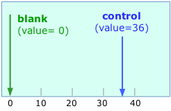
One measurement is done on a solution as similar to the unknowns as possible except that it contains no iron at all. This sample is called the blank. You adjust a control on the photometer to set its reading to zero when examining the blank.
The other measurement is made on a sample containing a known concentration of iron; this is usually called the control. You adjust the sensitivity of the photometer to produce a reading of some arbitrary value (50, say) with the control solution. Assuming the photometer reading is directly proportional to the concentration of iron in the sample (this might also have to be checked, in which case a calibration curve must be consructed), the photometer reading can then be converted into iron concentration by simple proportion.
Consider the two pairs of observations depicted here:
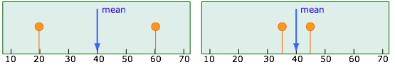
Notice that these two sample means happen to have the same value of “40” (pure luck!), but the difference in the precisions of the two measurements makes it obvious that the set shown on the right is more reliable. How can we express this fact in a succinct way? We might say that one experiment yields a value of 40 ±20, and the other 40 ±5. Although this information might be useful for some purposes, it is unable to provide an answer to such questions as "how likely would another independent set of measurements yield a mean value within a certain range of values?" The answer to this question is perhaps the most meaningful way of assessing the "quality" or reliability of experimental data, but obtaining such an answer requires that we employ some formal statistics.
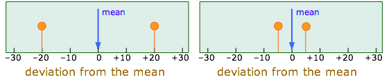
Deviations from the mean
We begin by looking at the differences between the sample mean and the individual data values used to compute the mean. These differences are known as deviations from the mean, xi–xm. These values are depicted below; note that the only difference from the plots above is placement of the mean value at 0 on the horizonal axis.
The variance and its square root
Next, we need to find the average of these deviations. Taking a simple average, however, will not distinguish between these two particular sets of data, because both deviations average out to zero. We therefore take the average of the squares of the deviations (squaring makes the signs of the deviations disappear so they cannot cancel out). Also, we compute the average by dividing by one less than the number of measurements, that is, by n–1 rather than by n. The result, usually denoted by S2, is known as the variance:
![]()
Finally, we take the square root of the variance to obtain the standard deviation S: